Catalogue

This notebook shows how you can examine statistical parameters of an earthquake catalogue and visualize it on a high-quality map.

import pandas as pd
import os
from IPython.display import Image, display
from openquake.plt.catalogue import visualize_catalogue

Descriptions of inputs and input files used here are briefly summarized below. For more detailed information, please see Data Format section.

• catalogue (str): Path to the HMTK-formatted CSV catalogue.

• polygon (str): Path to the GeoJSON file for the study area boundary.

• region (list): Map extent [West, East, South, North].

• output_png (str): Path to output image.

• bins (list): List of dictionaries containing magnitude bins and their formatting styles. Defaults to 3.5-4.5-5.5-6.5 binning scheme.

catalogue = "../data/cat_it.csv"
polygon = "../data/it_11in1_buffered.geojson"
output_map = "it_map.png"
it_region = [4, 22, 35, 48]
custom_bins = [
    {"min_mag": 3.5, "max_mag": 4.5, "color": "blue", "size": "0.08c"},
    {"min_mag": 4.5, "max_mag": 5.5, "color": "green", "size": "0.12c"},
    {"min_mag": 5.5, "max_mag": 6.5, "color": "orange", "size": "0.18c"},
    {"min_mag": 6.5, "max_mag": None, "color": "red", "size": "0.25c"}
]

Statistics of catalogue

This block loads the earthquake catalogue and generates a descriptive statistics table, including mean, standard deviation, and median, to provide an overview of the catalogue’s range and distribution.

df = pd.read_csv(catalogue)

# Generate descriptive statistics
summary_cols = ["magnitude", "depth", "year"]
stats_summary = df[summary_cols].describe().T
stats_summary['range'] = stats_summary['max'] - stats_summary['min']
stats_summary.columns = [
    'Count', 'Mean', 'Std Dev', 'Min', '25%', '50% (Median)', '75%', 'Max', 'Range'
]

print("Statistical Summary of the catalogue: ")
display(stats_summary.style.format("{:.2f}"))
print(f"\nTotal Number of Events: {len(df)}")
print(f"Time Span: {df['year'].min():.0f} to {df['year'].max():.0f} ({df['year'].max() - df['year'].min():.0f} years)")

Statistical Summary of the catalogue:

	Count	Mean	Std Dev	Min	25%	50% (Median)	75%	Max	Range
magnitude	7528.00	4.30	0.63	3.50	3.79	4.20	4.65	7.34	3.84
depth	7528.00	10.33	8.20	0.00	5.00	9.10	12.50	50.00	50.00
year	7528.00	1916.21	133.43	1005.00	1896.00	1963.00	2002.00	2020.00	1015.00

Total Number of Events: 7528
Time Span: 1005 to 2020 (1015 years)

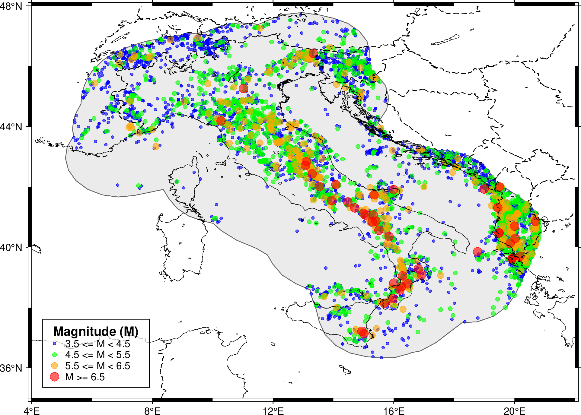
Catalogue visualization using GMT

The next block uses a plotting function that is available in the module openquake.plt.catalogue.

• This function provides a professional mapping interface for HMTK-formatted catalogues,

• Supports GeoJSON for boundary plotting,

• Bins earthquakes by magnitude for clear visualization,

• Produces publication-quality Generic Mapping Tools (GMT) [2] maps with legends and geographic layers.

output_dir = os.path.join("..", "output")
if not os.path.exists(output_dir):
    os.makedirs(output_dir)

file_name = "cat_it_map.png"
output_map = os.path.join(output_dir, file_name)

visualize_catalogue(
    catalogue=catalogue,
    polygon=polygon,
    region=it_region,
    output_png=output_map,
    bins=custom_bins
)

display(Image(filename=output_map))

Done! ../output/cat_it_map.png generated.