Gutenberg-Richter Recurrence Model Fitting

One of the fundamental components of Probabilistic Seismic Hazard Analysis (PSHA) is characterizing the seismicity of a source region by defining its Magnitude-Frequency Distribution (MFD). The MFD quantifies the expected annual rate of earthquakes exceeding a specific magnitude threshold.

The baseline mathematical framework for this analysis is the classic Gutenberg-Richter (G-R) recurrence law [10], expressed as:

\[\log_{10} N(M) = a - bM\]

Where:

N(M) is the cumulative annual rate of earthquakes with magnitudes greater than or equal to \(M\).
a-value represents the overall level of seismicity (productivity) of the zone.
b-value indicates the relative ratio of small to large earthquakes.

This notebook provides a workflow for analyzing an earthquake catalogue and fitting recurrence parameters using the OpenQuake Hazard Modeller’s Toolkit [1]. Specifically, we present two different algorithms to derive the Gutenberg-Richter parameters: Aki Maximum Likelihood and B-Value Maximum Likelihood (Both is available in openquake.hmtk.seismicity.occurrence).

[1]:

import pandas as pd
import numpy as np
import matplotlib.pyplot as plt
from openquake.hmtk.seismicity.catalogue import Catalogue
from openquake.hmtk.seismicity.occurrence.aki_maximum_likelihood import AkiMaxLikelihood
from openquake.hmtk.seismicity.occurrence.b_maximum_likelihood import BMaxLikelihood

Aki Maximum Likelihood (`AkiMaxLikelihood`)

Developed by Aki (1965) [11] and implemented here with the discrete bin-width correction by Bender (1983) [12], this method estimates the \(b\)-value using a Maximum Likelihood Estimation (MLE) approach.

While the original Aki formulation assumes a continuous magnitude distribution, earthquake catalogues group magnitudes into discrete bins (e.g., \(\Delta M = 0.1\)). To prevent statistical bias arising from this discretization, the code integrates Bender’s correction factor and formulates the calculation as:

\[b = \frac{\log_{10}e}{\bar{M} - M_{min} + \frac{\Delta M}{2}}\]

Where:

\(\mathbf{\bar{M}}\) (m_ave): The mean magnitude of the events that are equal to or greater than the completeness magnitude (\(M \geq M_c\)).
\(\mathbf{M_{min}}\) (m_min): The minimum discrete magnitude bin placeholder above or equal to \(M_c\) within the sample.
\(\mathbf{\Delta M}\) (dmag): The magnitude bin width interval (typically \(0.1\)).

The standard deviation (\(\sigma_b\)) of the estimated \(b\)-value is computed using the sample variance weighted by the number of observations per bin, following Bender’s uncertainty estimator:

\[\sigma_b = \ln(10) \cdot b^2 \cdot \sqrt{\frac{\sum (M_i - \bar{M})^2}{N(N - 1)}}\]

The required input for AkiMaxLikelihood algorithm is briefly described below. For more detailed information, please see Data Format section.

catalogue (str): Path to the HMTK-formatted CSV catalogue.
Mc: Completeness magnitude for the catalogue.

[2]:

df = pd.read_csv("../data/hmtk_sample_catalogue.csv")
Mc = 3.5

catalogue = Catalogue()
catalogue.data = {'magnitude': df['magnitude'].values, 'year': df['year'].values.astype(int)}
catalogue.end_year = int(df['year'].max())
end_year = int(catalogue.end_year)
start_year = int(catalogue.data['year'].min())
time_span = end_year - start_year + 1

print(f"Start year={start_year}, End year={end_year}, Time Span={time_span} years")

Start year=1, End year=10000, Time Span=10000 years

Below, you see how to obtain \(b\)-value, its sigma, and \(a\)-value.

[3]:

# b_val and sigma_b calculation
b_val, sigma_b = AkiMaxLikelihood().calculate(catalogue, completeness=Mc)

# a_val calculation
df_complete = df[df["magnitude"] >= Mc]
neq_complete = len(df_complete)

# Annualized earthquake rate (N_cumulative / T)
annual_rate = neq_complete / time_span
a_val = np.log10(annual_rate) + b_val * Mc

print(f"Results: a={a_val:.3f}, b={b_val:.3f} ±{sigma_b:.3f}")

Results: a=3.881, b=0.888 ±0.004

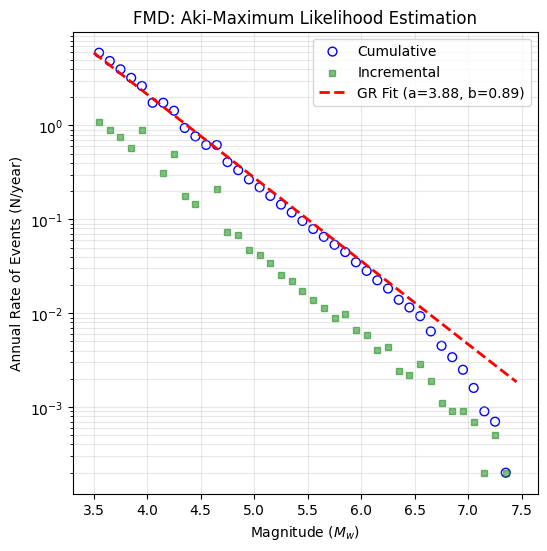
You can plot the FMD using obtained GR parameters, and catalogue.

[4]:

# Plot FMD
bins = np.arange(df["magnitude"].min(), df["magnitude"].max() + 0.1, 0.1)
hist, edges = np.histogram(df["magnitude"], bins=bins)
cum_evars = np.cumsum(hist[::-1])[::-1]
m_model = np.linspace(Mc, df["magnitude"].max(), 100)
v_model = 10 ** (a_val - b_val * m_model)

# Plot
plt.figure(figsize=(6, 6))
plt.scatter(edges[:-1], cum_evars / time_span, s=40, facecolors='none', edgecolors='b', label="Cumulative")
plt.scatter(edges[:-1], hist / time_span, s=20, color="g", marker="s", alpha=0.5, label="Incremental")
plt.plot(m_model, v_model, "r--", linewidth=2, label=f"GR Fit (a={a_val:.2f}, b={b_val:.2f})")
plt.yscale("log")
plt.xlabel("Magnitude ($M_w$)")
plt.ylabel("Annual Rate of Events (N/year)")
plt.title("FMD: Aki-Maximum Likelihood Estimation")
plt.grid(True, which="both", alpha=0.3)
plt.legend()
plt.show()

GR parameters with Time-Varying Completeness (`BMaxLikelihood`)

BMaxLikelihood algorithm enables an advanced extension based on Utsu (1965) [13], Weichert (1980) [14], and Bender (1983) [12] that accounts for both magnitude binning/discretization effects and time-varying magnitude completeness (Mc).

Historical catalogues are inherently non-homogeneous because seismic networks improve over time; smaller earthquakes are fully captured in recent years, whereas only larger events were recorded in the past. Treating such a partitioned catalogue with a completeness magnitude leads to systematic bias in Gutenberg-Richter parameters.

The BMaxLikelihood operates by partitioning the catalogue into distinct temporal windows based on a completeness table (defined by cut-off years \(T_i\) and corresponding magnitudes \(M_{c,i}\)).

For each chronological interval, the BMaxLikelihood isolates compliant events and invokes an underlying Aki MLE sub-routine with Bender’s bin-width (\(\Delta M\)) correction:

\[b_i = \frac{\log_{10}e}{\bar{M}_i - M_{min,i} + \frac{\Delta M}{2}}\]

Once local \(b\)-values (\(b_i\)) and their uncertainties (\(\sigma_{b,i}\)) are stacked for all valid intervals, a single unified \(b_{final}\) is derived using a statistical ensemble approach defined in the configuration (Weighted or Harmonic mean):

\[b_{final} = \sum_{i=1}^{k} \left( b_i \cdot \frac{N_i}{N_{total}} \right)\]

Where \(N_i\) is the number of events in the \(i\)-th temporal completeness block.

Unlike the AkiMaxLikelihood, BMaxLikelihood jointly solves for the annualized productivity parameter (\(a\)-value) using the maximum likelihood solution for multi-period data formulated by Weichert (1980) [14] and McGuire (2004) [15].

\[\lambda(M_{min}) = \frac{\sum_{i=1}^{k} N_i}{\sum_{i=1}^{k} \left( T_i \cdot e^{-\beta M_j} \right)}\]

Where \(T_i\) represents the seismic observation duration (years) for each interval, and \(\beta = b_{final} \cdot \ln(10)\). The calculated scalar is then mapped back to the baseline minimum magnitude (\(M_{min}\)) to compute the annualized \(a\)-value:

\[a = \log_{10}(\lambda(M_{min})) + b_{final} \cdot M_{min}\]

The BMaxLikelihood requires specific data structures and configuration parameters to handle time-varying completeness.

catalogue: An instance of the HMTK Catalogue object containing the earthquake database (specifically requires magnitude and year attributes).
completeness (numpy.ndarray): A 2D completeness matrix/table structured as [[year_1, Mc_1], [year_2, Mc_2], ...]. It defines the chronological cut-off thresholds where specific magnitude ranges become statistically complete.
config (dict): A configuration dictionary containing the execution hyper-parameters:
- Average Type (str): Method used to ensemble the multi-period recurrence trends. Options are "Weighted" (proportional to event-counts per window, recommended) or "Harmonic" mean.
- magnitude_interval (float): The magnitude bin width or rounding increment used in the catalog (typically 0.1), critical for Bender’s discretization correction.
- completeness (bool): Set to True to activate multi-period analysis.
- reference_magnitude (float):
  - If set to 0.0 or None, the module executes standard Gutenberg-Richter reporting and returns the annualized \(a\)-value, \(b\)-value, and their respective uncertainties.
  - If a specific engineering design magnitude is provided (e.g., \(M_w = 5.0\)), the algorithm bypasses standard parameter reporting and outputs the calculated annual exceedance rate (\(\lambda\)) and its variance for that exact threshold.

[5]:

bin_w = 0.1
Mc = 3.5
start_year = int(df["year"].min())
end_year = int(catalogue.end_year)
total_years = end_year - start_year + 1
completeness = np.array([[start_year, Mc]])

# Config
config = {
    "Average Type": "Weighted",
    "reference_magnitude": 0.0,
    "magnitude_interval": bin_w,
    "completeness": True
}

[6]:

# b_val, sigma_b, a_val, and sigma_a calculation
b_val, sigma_b, a_val, sigma_a = BMaxLikelihood().calculate(catalogue, config, completeness)
print(f"Results: a={a_val:.3f} ±{sigma_a:.3f}, b={b_val:.3f} ±{sigma_b:.3f}")

--- ctime 1.0  m_c 3.5
Results: a=3.881 ±0.013, b=0.888 ±0.004

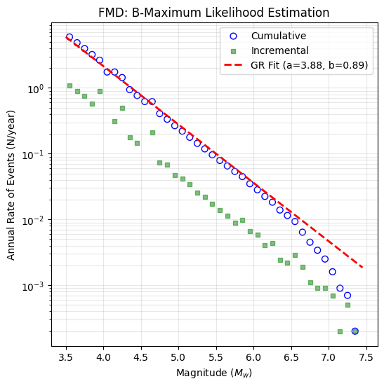
[7]:

# Plot FMD
m_bins = np.arange(df["magnitude"].min(), df["magnitude"].max() + bin_w, bin_w)
hist, edges = np.histogram(df["magnitude"], bins=m_bins)
cum_events = np.cumsum(hist[::-1])[::-1]
m_model = np.linspace(Mc, df["magnitude"].max(), 100)
gr_model_total = (10 ** (a_val - b_val * m_model))

# Plot
plt.figure(figsize=(6, 6))
plt.scatter(edges[:-1], cum_events / total_years, s=40, facecolors='none', edgecolors='b', label="Cumulative")
plt.scatter(edges[:-1], hist / total_years, s=20, color="g", marker="s", alpha=0.5, label="Incremental")
plt.plot(m_model, gr_model_total, "r--", linewidth=2, label=f"GR Fit (a={a_val:.2f}, b={b_val:.2f})")
plt.yscale("log")
plt.xlabel("Magnitude ($M_w$)")
plt.ylabel(f"Annual Rate of Events (N/year)")
plt.title("FMD: B-Maximum Likelihood Estimation")
plt.grid(True, which="both", alpha=0.3)
plt.legend()
plt.show()

Gutenberg-Richter Recurrence Model Fitting

Aki Maximum Likelihood (AkiMaxLikelihood)

GR parameters with Time-Varying Completeness (BMaxLikelihood)

Aki Maximum Likelihood (`AkiMaxLikelihood`)

GR parameters with Time-Varying Completeness (`BMaxLikelihood`)